Domain Generalization Tutorials - Part 1

👋 Hi there. I’m Khiem. Welcome to my page, where I gather and share some intuitive explanations and hands-on tutorials on a range of topics in AI.

🚀 I am going to kick off this website with a series of tutorials about the topic of Domain Generalization. This series provides a systematic survey of outstanding methods in literature and my own implementations to demonstrate these methods. This is the first part of the series that gives you a brief understanding of the term Domain Generalization. Let’s get started.

1. Background

Motivation

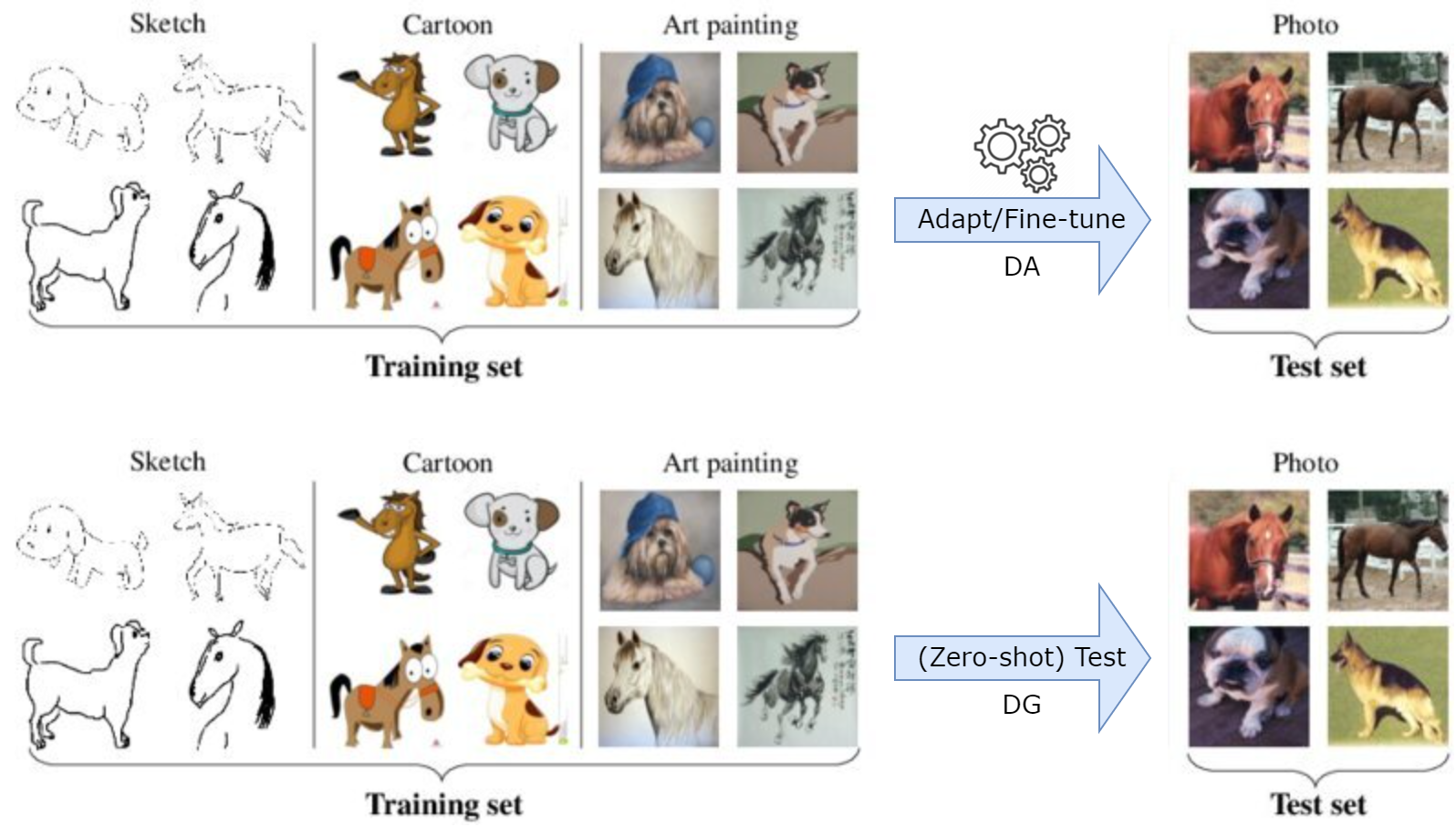
Machine Learning (ML) systems generally rely on an over-simplified assumption, that is, the training (source) and testing (target) data are independent and identically distributed (i.i.d.), however, this assumption is not always true in practice. When the distributions of training data and testing data are different, which is referred to as the domain shift problem, the performance of these ML systems often catastrophically decreases due to domain distribution gaps. Moreover, in many applications, target data is difficult to obtain or even unknown before deploying the model. For example, in biomedical applications where data differs from equipment to equipment and institute to institute, it is impractical to collect the data of all possible domains in advance.

To address the domain shift problem, as well as the absence of target data, the topic of Domain Generalization (DG) was introduced. Specifically, the goal in DG is to learn a model using data from a single or multiple related but distinct source domains in such a way that the model can generalize well to any unseen target domain.

Watch out! Unlike other related topics such as Domain Adaptation (DA) or Transfer Learning (TL), where the ML models can do some forms of adaptation on target data, DG considers more ubiquitous scenarios in practice where target data is inaccessible during model learning.

Figure 1. Examples from the PACS dataset for DG. Adapted from [1].

Formulation

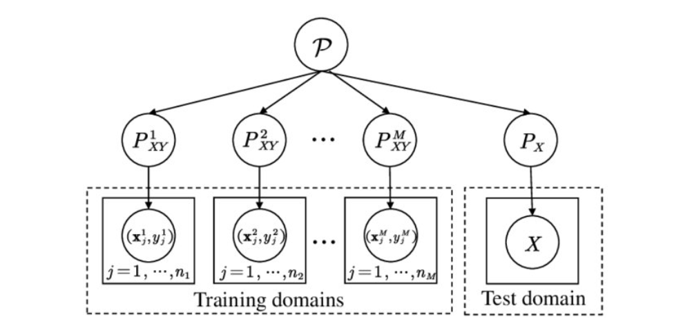
In the context of DG, we have access to $M$ similar but distinct source domains \(S_{source}=\{S_m=\{(x, y)\}\}_{m=1}^M\), each associated with a joint distribution \(P_{XY}^{(m)}\) with:

• \(P_{XY}^{(m)}\neq P_{XY}^{({m}')}\) with \(m\neq {m}'\) and \(m, {m}'\in \{1, ..., M\}\)
• \(P_{Y\mid X}^{(m)}= P_{Y\mid X}^{({m}')}\) with \(m\neq {m}'\) and \(m, {m}'\in \{1, ..., M\}\)

and we have to minimize prediction error on an unseen target domain \(S_{target}\) with:

• \(P_{XY}^{(target)}\neq P_{XY}^{(m)}\) with \(m\in \{1, ..., M\}\)
• \(P_{Y\mid X}^{(target)}= P_{Y\mid X}^{(m)}\) with \(m\in \{1, ..., M\}\)

Figure 2. Illustration of DG. Adapted from [1].

2. Tutorial Settings

In this series of tutorials, besides introducing and explaining outstanding DG methods intuitively, I also prepare those implementations and practice them on a real-world problem, which is classifying cardiac abnormalities from twelve-lead ECGs (see more details in PhysioNet Challenge 2021). This can help you understand better as well as apply these methods to your own problems immediately.

Datasets

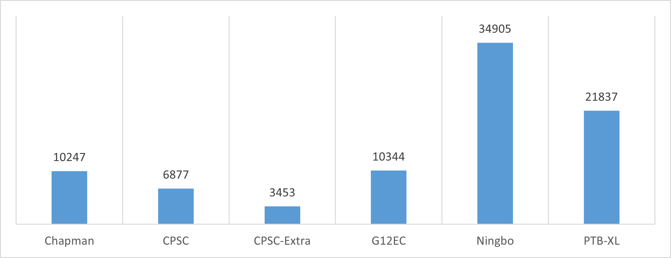
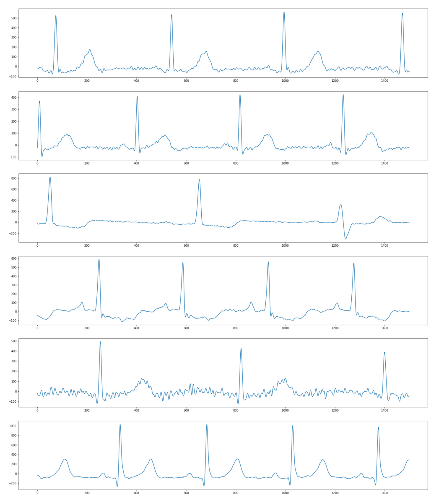
The datasets are from PhysioNet Challenge 2021, containing twelve-lead ECG recordings from 6 institutes in 4 countries across 3 continents. Each recording was annotated with one or more of 26 types of cardiac abnormalities, which means the problem is multi-label classification. Figure 3 shows the number of data samples in each dataset, and Figure 4 illustrates the difference in the appearance of signals from 6 institutes.

Figure 3. The number of data samples in each dataset.

Figure 4. The difference in the appearance of signals from 6 institutes.

I recommend you read some documents to understand what is ECG and cardiac abnormalities, as well as our problem:

• https://en.wikipedia.org/wiki/Electrocardiography
• https://www.who.int/health-topics/cardiovascular-diseases
• https://arxiv.org/abs/2207.12381

Important things to remember about our problem:

• Input: twelve 1D-signals, a matrix with a shape of (12, 5000)
• Output: one or more of 26 classes, a vector of 26 elements, each 0 or 1

Baseline

We always need a baseline model before applying any advanced methods. Here, I use:

• One-dimensional SEResNet34 model
• Cross Entropy Loss function
• Adam optimizer with lr = 1e-3 and weight_decay = 5e-5
• Cosine Annealing scheduler with eta_min = 1e-4 and T_max = 50
• The batch size is 512 and the number of epochs is 80

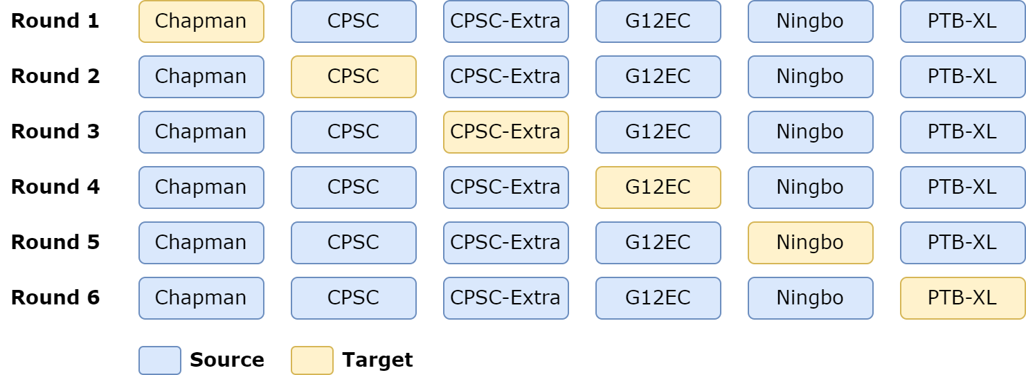
Evaluation of DG algorithms often follows the leave-one-domain-out rule. It leaves one dataset as the target domain while treating the others as the training part, i.e., source domains. Based on this evaluation strategy, the baseline model’s performance is shown in the table below:

Figure 5. Leave-one-domain-out evaluation strategy.

	Chapman	CPSC	CPSC-Extra	G12EC	Ningbo	PTB-XL	Avg
Baseline	0.4290	0.1643	0.2067	0.3809	0.3987	0.3626	0.3237

Now we are ready to start exploring DG methods, next part of the series will present the first approach.

References

[1] Generalizing to Unseen Domains: A Survey on Domain Generalization
[2] Domain Generalization: A Survey