Domain Generalization Tutorials - Part 2

👋 Hi there. Welcome back to my page, this is part 2 of my tutorial series about the topic of Domain Generalization (DG). In this article, I will introduce the first approach to the DG problem, which I call conventional generalization.

1. Conventional Generalization

Conventional generalization methods such as data augmentation or weight decay aim to make ML models less overfit on training data, therefore these models after training are assumpted to generalize well on testing data regardless of its domain. This is a great starting point to approach the DG problem. Despite the popularity of data augmentation and weight decay, I will present two more advanced and effective methods, multi-task learning and flat minima seeking.

2. Multi-task Learning

Motivation

The goal of multi-task learning (with deep neural networks) is to jointly learn one or more sub-tasks beside the main task using a shared model, therefore facilitating the model’s shared representations to be generic enough to deal with different tasks, eventually reducing overfitting on the main task. In general, sub-tasks for performing multi-task learning are defined based on specific data and problems. After that, jointly learning is established by minimizing a joint loss function.

Multi-task learning is popular in ML literature but rarely realized. For example, in Computer Vision, Object Detection aims to localize and classify objects simultaneously. In Natural Language Processing, Intent Detection and Slot Filling aims to simultaneously identify the speaker’s intent from a given utterance and extract from the utterance the correct argument value for the slots of the intent.

Method

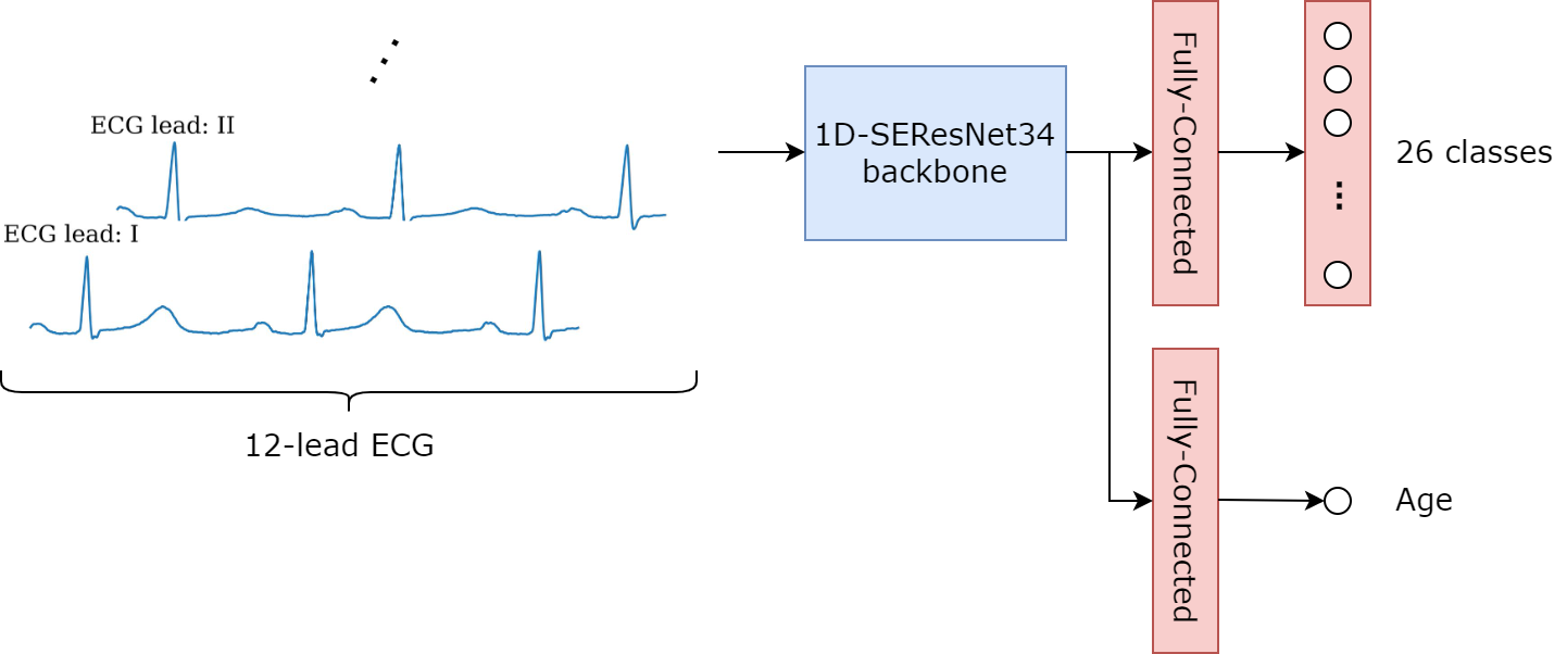
As mentioned before, sub-tasks for performing multi-task learning are defined based on specific data and problems. In our ECGs-based cardiac abnormalities classification problem, I define and perform a sub-task of age regression (AgeReg) from ECGs, which is feasible from a medical perspective. Figure 1 illustrates the architecture of the model and Snippet 1 describes the auxiliary module which performs regression.

Figure 1. Multi-task learning architecture.

"""
Snippet 1: Age Regression module. 
"""
import torch.nn as nn

class SEResNet34(nn.Module):
  ...
  self.auxiliary = nn.Sequential(
    nn.Dropout(0.2), 
    nn.Linear(512, 1), 
  )
  ...

  def forward(self, inputs):
    ...
    return self.classifier(feature), self.auxiliary(feature)

For optimization, I use cross-entropy loss for the main classification task and L1 loss for the regression sub-task. The second loss is added to the main loss with an auxiliary_lambda hyperparameter, which is set to 0.02. Snippet 2 describes the optimization process. All other settings are similar to the baseline in the previous article.

"""
Snippet 2: Optimization process. 
"""
import torch.nn.functional as F

...
logits, sub_logits = model(ecgs)
loss, sub_loss = F.binary_cross_entropy_with_logits(logits, labels), F.l1_loss(sub_logits, ages)
(loss + auxiliary_lambda*sub_loss).backward()
...

3. Flat Minima Seeking

Motivation

In optimization, the connection between different types of local optima and generalization has been explored extensively in many studies [2]. These studies show that sharp minima often lead to larger test errors while flatter minima yield better generalization. This finding raised a new research direction in deep learning that seeks out flatter minima when training neural networks.

The two most popular flatness-aware solvers are Sharpness-Aware Minimization (SAM) and Stochastic Weight Averaging (SWA). SAM is a procedure that simultaneously minimizes loss value and loss sharpness, this procedure finds flat minima directly but also doubles training cost. Meanwhile, SWA finds flat minima by a weight ensemble approach and has almost no computational overhead.

Method

Intuitively, SWA updates a pre-trained model (namely, a model trained with sufficiently enough training epochs, $K_0$) with a cyclical or high constant learning rate scheduling. SWA gathers model parameters for every $K$ epoch during the update and averages them for the model ensemble. SWA finds an ensembled solution of different local optima found by a sufficiently large learning rate to escape a local minimum.

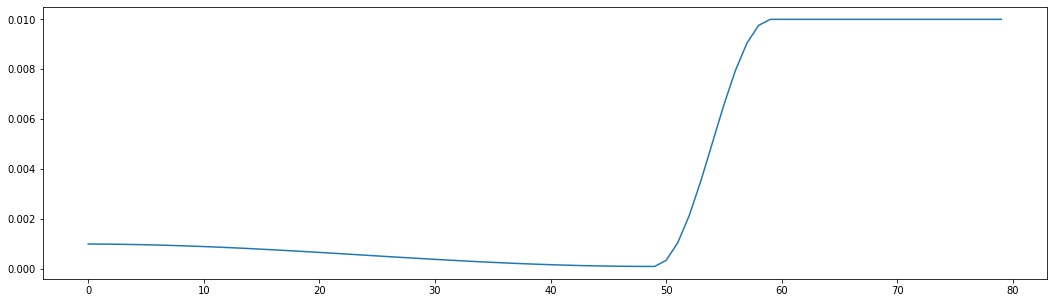
Since 2020, SWA was included in PyTorch effectively. We need two ingredients to apply SWA to our model, a swa_model and a swa_scheduler. Snippet 3 illustrates how to initialize these two entities in PyTorch. Figure 2 shows the whole learning rate schedule during training, where $K_0$ is set to T_max of the base scheduler.

"""
Snippet 3: Initializing swa_model and swa_scheduler. 
"""
import torch.optim as optim

...
swa_model = optim.swa_utils.AveragedModel(model)
swa_scheduler = optim.swa_utils.SWALR(
  optimizer, swa_lr = 1e-2, 
  anneal_strategy = "cos", anneal_epochs = 10, 
)
...

Figure 2. Learning rate schedule during training.

Snippet 4 below briefs the training loop. It is a little bit tricky when applying SWA to ML models that have BatchNorm layers, we need to use a utility function update_bn to compute the BatchNorm statistics for the SWA model on a given data loader.

"""
Snippet 4: Training loop. 
"""
for epoch in range(1, num_epochs + 1):
...
  if not epoch > scheduler.T_max:
    scheduler.step()
  else:
    swa_model.update_parameters(model.train())
    swa_scheduler.step()
...

...
optim.swa_utils.update_bn(loaders["train"], swa_model)
...

4. Results

The table below shows the performance of the two presented methods in this article:

	Chapman	CPSC	CPSC-Extra	G12EC	Ningbo	PTB-XL	Avg
Baseline	0.4290	0.1643	0.2067	0.3809	0.3987	0.3626	0.3237
AgeReg	0.4222	0.1715	0.2136	0.3923	0.4024	0.4021	0.3340
SWA	0.4271	0.1759	0.2052	0.3969	0.4313	0.4203	0.3428

To be continued …

References

[1] Multi-task Learning with Deep Neural Networks: A Survey
[2] On Large-Batch Training for Deep Learning: Generalization Gap and Sharp Minima
[3] Sharpness-Aware Minimization for Efficiently Improving Generalization
[4] Averaging Weights Leads to Wider Optima and Better Generalization
[5] SWAD: Domain Generalization by Seeking Flat Minima