Domain Generalization Tutorials - Part 3

👋 Hi there. Welcome back to my page, this is part 3 of my tutorial series about the topic of Domain Generalization (DG). From this article, we will explore domain-aware approaches which take the problem domain shift into account. Today, I introduce the first family of methods which is inter-domain data augmentation.

1. Inter-domain Data Augmentation

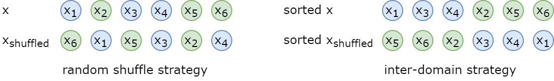
Mixing data augmentation is an emerging type of augmentation method that has shown superior in recent years. The methods of this type do a convex combination (mix) on two data instances at the input or feature level, hence generating a new instance for training ML models. Differing from conventional data augmentation such as crop, scale, or cut out which preserves the context of the original instance, mixing augmentation creates instances with new contexts, in other words, new domains, this is extremely suitable for solving the DG problem. Because these methods perfectly fit into mini-batch training, we have two ways to select data instances for doing the mixing, without domain labels (random shuffle mixing) and with domain labels (inter-domain mixing). Figure 1 illustrates these selection strategies. Let’s dive into Mixup and MixStyle, the two most popular and effective augmentation methods for DG.

Figure 1. Illustration of mixing strategies. Adapted from [2].

2. Mixup

As mentioned above, Mixup perfectly fits into mini-batch training, at each training iteration, we select two instances in a mini-batch following a given strategy (random shuffle or inter-domain) and then mix them at the input level through a convex combination to generate a new instance:

\[x_{mix} = \lambda x + (1-\lambda ) x_{shuffled}\]

where $\lambda$ is drawn from a Beta distribution $\lambda \sim Beta(\alpha , \alpha )$ with $\alpha \in (0, \infty )$ is a hyper-parameter.

We also have to create the label for the generated instance by mixing labels of original instances in the same way:

\[y_{mix} = \lambda y + (1-\lambda ) y_{shuffled}\]

The above combination of original labels can yield a non-integer label for the generated instances, this is not fit with the classification problem which requires the label must be categorical. Therefore, we have to do a trick, mixing loss instead of mixing labels:

\[loss = \lambda loss(logit_{mix}, y) + (1-\lambda ) loss(logit_{mix}, y_{shuffled})\]

where $logit_{mix}$ is output from the model of $x_{mix}$.

Snippet 1 describes how to integrate Mixup into the training pipeline.

"""
Snippet 1: Mixup integration. 
"""
import random
import pandas, numpy as np
import torch

...
if random.random() < 0.5:
  logits = model(ecgs)
  loss = F.binary_cross_entropy_with_logits(logits, labels)
else:
  shuffled_indices = torch.randperm(ecgs.size()[0])
  mixup_lambda = np.random.beta(0.2, 0.2)
  logits = model(mixup_lambda*ecgs + (1 - mixup_lambda)*ecgs[permuted_indices])
  loss = mixup_lambda*F.binary_cross_entropy_with_logits(logits, labels) + (1 - mixup_lambda)*F.binary_cross_entropy_with_logits(logits, labels[permuted_indices])
...

3. MixStyle

Unlike Mixup which creates new instances at the input level, MixStyle is a recent method that generates new instances in the feature space by mixing their “styles”. The style of an instance is represented in its feature statistics which are mean and standard deviation across spatial dimensions in the feature space. At each iteration, we select two instances in a mini-batch following a given strategy (random shuffle or inter-domain) and then mix their styles in a similar way as Mixup:

\[\mu _{mix} = \lambda \mu (x) + (1-\lambda ) \mu (x_{shuffled})\] \[\sigma _{mix} = \lambda \sigma (x) + (1-\lambda ) \sigma (x_{shuffled})\]

where $\mu$ and $\sigma$ are mean and standard deviation operations, respectively. $\lambda \sim Beta(\alpha , \alpha )$ with $\alpha \in (0, \infty )$ is a hyper-parameter.

Finally, the mixed feature statistics are applied to the style-normalized $x$:

\[MixStyle(x) = \sigma _{mix}\frac{x - \mu (x)}{\sigma (x)} + \mu _{mix}\]

If you look at the above formula carefully, you can realize that MixStyle does not actually create a new instance, but mixes the style of an instance into another one to make it become “new”. Therefore, MixStyle uses the original label $y$ of this “new” instance $x$.

Similar to Mixup, MixStyle is easy to implement, but where to apply MixStyle? Experiments showed that applying MixStyle after the first three residual blocks in a ResNet-like model gives the best results in our problem. Snippet 2 illustrates this setting.

"""
Snippet 2: MixStyle setting. 
"""
import torch.nn as nn

class SEResNet34(nn.Module):
  ...
  self.augment = MixStyle(alpha = 0.1, p = 0.5)
  ...

  ...
  self.stem = ...
  self.stage_0 = ...

  self.stage_1 = ...
  self.stage_2 = ...
  self.stage_3 = ...
  ...

  def forward(self, inputs, augment = False):
    ...
    feature = self.stem(inputs)
    feature = self.augment(self.stage_0(inputs), activate = augment)

    feature = self.augment(self.stage_1(inputs), activate = augment)
    feature = self.augment(self.stage_2(inputs), activate = augment)
    feature = self.stage_3(inputs)
    ...

4. Results

The table below shows the performance of the two presented methods in this article:

	Chapman	CPSC	CPSC-Extra	G12EC	Ningbo	PTB-XL	Avg
Baseline	0.4290	0.1643	0.2067	0.3809	0.3987	0.3626	0.3237
AgeReg	0.4222	0.1715	0.2136	0.3923	0.4024	0.4021	0.3340
SWA	0.4271	0.1759	0.2052	0.3969	0.4313	0.4203	0.3428
Mixup	0.4225	0.1759	0.2127	0.3901	0.4025	0.3934	0.3329
MixStyle	0.4253	0.1681	0.2027	0.3927	0.4117	0.3853	0.3310

To be continued …

References

[1] Mixup: Beyond Empirical Risk Minimization
[2] Domain Generalization with MixStyle