Domain Generalization Tutorials - Part 4

👋 Hi there. Welcome back to my page, this is part 4 of my tutorial series about the topic of Domain Generalization (DG). This article will cover the approach of domain alignment, to which most existing DG methods belong. In addition, we also cover an improvement upon this approach.

1. Domain Alignment

The central idea of domain alignment is to minimize the difference among source domains for learning domain-invariant representations. The motivation is straightforward: features that are invariant to the source domains should also generalize well on any unseen target domain. Traditionally, the difference among source domains is modeled by Feature Correlation or Maximum Mean Discrepancy, these entities are minimized to learn domain-invariant representations. However, let’s explore simpler and more effective domain alignment methods.

2. Domain-Adversarial Training

Motivation

Don’t be afraid to see the word “adversarial”, this method is simple to understand if you have read about multi-task learning in part 2 of the series, but if not, it’s still simple. Domain-adversarial training (DAT) perfectly represents the spirit of the domain alignment approach, that is to learn the feature cannot tell which source domain the instance came from.

By leveraging a multi-task learning setting, DAT combines discriminativeness and domain-invariance into the same representations. To this end, a subtle trick is introduced along with the main method.

Method

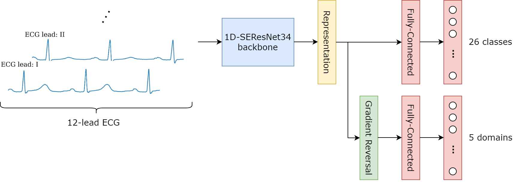
Specifically, along the main task of cardiac abnormalities classification, DAT performs a subtask of domain identification and uses a gradient reversal layer to learn the representations in an adversarial manner. Figure 1 illustrates the architecture of the model and Snippet 1 describes the auxiliary module which performs DAT.

Figure 1. Domain-adversarial training architecture.

"""
Snippet 1: DAT module. 
"""
import torch.nn as nn

class SEResNet34(nn.Module):
  ...
  self.auxiliary = nn.Sequential(
    GradientReversal(), 
    nn.Dropout(0.2), 
    nn.Linear(512, num_domains), 
  )
  ...

  def forward(self, inputs):
    ...
    return self.classifier(feature), self.auxiliary(feature)

The model is optimized with a combined loss similar to multi-task learning. Snippet 2 describes the optimization process.

"""
Snippet 2: Optimization process. 
"""
import torch.nn.functional as F

...
logits, sub_logits = model(ecgs)
loss, sub_loss = F.binary_cross_entropy_with_logits(logits, labels), F.cross_entropy(sub_logits, domains)
(loss + auxiliary_lambda*sub_loss).backward()
...

Intuitively, the gradient reversal layer is skipped in the forward pass and just flips the sign of the gradient flow through it during the backpropagation process. Look at the position of this layer, it is placed right before the domain classifier $g_{d}$, this means that during training, $g_{d}$ is updated with $\frac{\partial L_{sub}}{\partial \theta_{g_d}}$ while the backbone $f$ is updated with $-\frac{\partial L_{sub}}{\partial \theta_{f}}$. In this way, the domain classifier learns how to use representations to identify the source domain of instances, but gives the reversed information to the backbone, forcing $f$ to generate domain-invariant representations.

3. Instance-Batch Normalization Network

Motivation

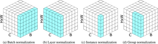
Nowadays, normalization layers are an important part of any neural network. There are many types of normalization techniques and each of them has its own characteristics and advantages, perhaps you have seen Figure 2 somewhere. We will talk about batch normalization (BN) and instance normalization (IN) here because of their effects on DG.

Figure 2. Different normalization techniques.

Although BN generally works well in a variety of tasks, it consistently degrades performance when it is trained in the presence of a large domain divergence. This is because the batch statistics overfit the particular training domains, resulting in poor generalization performance in unseen target domains. Meanwhile, IN does not depend on batch statistics. This property allows the network to learn feature representations that less overfit a particular domain. The downside of IN, however, is that it makes the features less discriminative with respect to instance categories, which is guaranteed in BN in contrast. Instance-Batch normalization (I-BN) is a mixture of BN and IN, which is introduced to reap the benefits of IN of learning domain-invariant representations while maintaining the ability to capture discriminative representations from BN.

Method

Snippet 3 is a simple implementation of a one-dimensional I-BN layer, just half of BN and half of IN. It is straightforward to extend the implementation to higher-dimension usages.

"""
Snippet 3: I-BN layer. 
"""
import torch
import torch.nn as nn

class Instance_BatchNorm1d(nn.Module):
  def __init__(self, num_features):
    super(Instance_BatchNorm1d, self).__init__()

    self.half_num_features = num_features//2
    self.BN, self.IN = nn.BatchNorm1d(num_features - self.half_num_features), nn.InstanceNorm1d(self.half_num_features, affine = True)

  def forward(self, input):
    half_input = torch.split(input, self.half_num_features, dim = 1)
    half_BN, half_IN = self.BN(half_input[0].contiguous()), self.IN(half_input[1].contiguous())

    return torch.cat((half_BN, half_IN), dim = 1)

But where to place I-BN layers in a specific network, a ResNet-like model for example? Another observation showed that, for BN-based CNNs, the feature divergence caused by appearance variance (domain shift) mainly lies in the shallow half of the CNN, while the feature discrimination for categories is high in deep layers, but also exists in shallow layers. Therefore, an original ResNet can is modified as follows to become an I-BN ResNet:

• Only use I-BN layers in the first three residual blocks and leave the fourth block as normal (similar to MixStyle in the previous article)
• For each selected block, only replace the BN layer after the first convolution layer in the main path with an I-BN layer

Snippet 4 illustrates this setting.

"""
Snippet 4: I-BN ResNet setting. 
"""
import torch.nn as nn

class SEResNet34(nn.Module):
  ...
  self.block = I_NBSEBlock()
  ...

  ...
  self.stem = ...
  self.stage_0 = nn.Sequential(
    self.block(i_bn = True), 
    self.block(i_bn = True), 
    self.block(i_bn = True), 
  )

  self.stage_1 = nn.Sequential(
    self.block(i_bn = True), 
    self.block(i_bn = True), 
    self.block(i_bn = True), 
    self.block(i_bn = True), 
  )
  self.stage_2 = nn.Sequential(
    self.block(i_bn = True), 
    self.block(i_bn = True), 
    self.block(i_bn = True), 
    self.block(i_bn = True), 
    self.block(i_bn = True), 
    self.block(i_bn = True), 
  )
  self.stage_3 = nn.Sequential(
    self.block(i_bn = False), 
    self.block(i_bn = False), 
    self.block(i_bn = False), 
  )
  ...

4. Domain-Specific I-BN Network

Motivation

Domain alignment methods generally have a common limitation, which will be discussed and addressed here. Look back to an illustration of DG from part 1, where a classifier trained in sketch, cartoon, art painting images encounters instances from a novel domain photo at test-time.

Figure 3. Examples from the PACS dataset for DG. Adapted from [1].

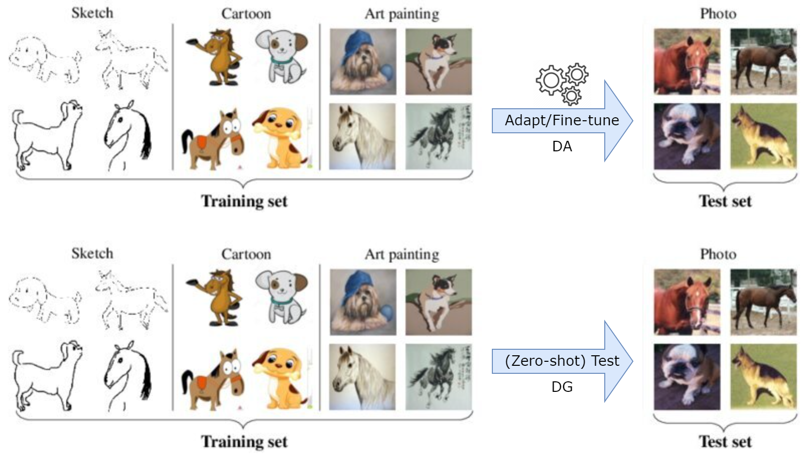
It is reasonable to note that leveraging the relative similarity of the photo instances to instances from art painting might result in better predictions compared to a setting where the model relies solely on invariant characteristics across domains. Both covered methods try to learn domain-invariant representations while ignoring domain-specific features, features that are specific to individual domains.

Extending from the above I-BN Net, domain-specific I-BN Net (DS I-BN Net) is developed which aims to capture both domain-invariant and domain-specific features from multi-source domain data.

Method

In particular, an original ResNet can is modified to become a DS I-BN ResNet in the following two steps:

• Turn all BN layers in the model into domain-specific BN (DSBN) modules
• Replace BN layers with I-BN layers at the same positions as I-BN ResNet

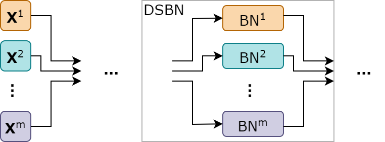
What is the DSBN? DSBN is a module that consists of $M$ BN layers, using parameters of each BN layer to capture domain-specific features of each individual domain in $M$ source domains. Specifically, during training, instances from domain $m$, $\mathbf{X}^{m}$ only go through the $m^{th}$ BN layer in the DSBN module. Figure 4 illustrates the module and Snippet 5 is its implementation in a one-dimensional version.

Figure 4. Domain-specific batch normalization module architecture.

"""
Snippet 5: I-BN layer. 
"""
import torch
import torch.nn as nn

class DomainSpecificBatchNorm1d(nn.Module):
  def __init__(self, num_features, num_domains):
    super(DomainSpecificBatchNorm1d, self).__init__()

    self.num_domains = num_domains
    self.BNs = nn.ModuleList(
      [nn.BatchNorm1d(num_features) for _ in range(self.num_domains)]
    )

  def forward(self, input, domains, is_training = True, running_domain = None):
    domain_uniques = torch.unique(domains)

    if is_training:
      outputs = [self.BNs[i](input[domains == domain_uniques[i]]) for i in range(domain_uniques.shape[0])]
      return torch.concat(outputs)
    else:
      output = self.BNs[running_domain](output)
      return output

At inference time, a test instance is fed into all $M$ “sub-networks” of all domains to get $M$ logits. The final logit is averaged over these $M$ logits and made the prediction.

5. Results

The table below shows the performance of the two presented methods in this article:

	Chapman	CPSC	CPSC-Extra	G12EC	Ningbo	PTB-XL	Avg
Baseline	0.4290	0.1643	0.2067	0.3809	0.3987	0.3626	0.3237
AgeReg	0.4222	0.1715	0.2136	0.3923	0.4024	0.4021	0.3340
SWA	0.4271	0.1759	0.2052	0.3969	0.4313	0.4203	0.3428
Mixup	0.4225	0.1759	0.2127	0.3901	0.4025	0.3934	0.3329
MixStyle	0.4253	0.1681	0.2027	0.3927	0.4117	0.3853	0.3310
DAT	0.4282	0.1712	0.1966	0.3956	0.4114	0.3878	0.3318
I-BN	0.4252	0.1748	0.2045	0.3817	0.4193	0.4161	0.3369
DS I-BN	0.4484	0.1805	0.2191	0.4318	0.3916	0.4242	0.3493

To be continued …

References

[1] Domain Generalization: A Survey
[2] Domain-Adversarial Training of Neural Networks
[3] Two at Once: Enhancing Learning and Generalization Capacities via IBN-Net
[4] Learning to Optimize Domain Specific Normalization for Domain Generalization
[5] Learning to Balance Specificity and Invariance for In and Out of Domain Generalization