


Easy Object Detection
From Classification to Detection with YOLO
👋 Hi there. Welcome back to my page. In the last 2 tutorial series on Domain Generalization and Federated Learning on IoT Devices, we dealt with 2 different types of classification (ECG classification and image classification), the most fundamental (and simple) task in Machine Learning (ML). Today, we will explore how to easily move from classification to object detection, a more advanced task in ML and Computer Vision (CV). Let’s get started.
1. Background
Motivation
I start this tutorial series and an open-source repository ezdet by 3 observations:
- When people begin to learn ML, specifically CV, they typically begin with an image classification tutorial, such as PyTorch’s one. After that, they usually move to the object detection problem next, where the difficulty occurs. In particular, the tutorial on object detection in the community is not good and dissimilar from the one on classification. Therefore, people come to some open-source repositories like YOLO from Ultralytics or Detectron. Although these repositories are powerful, they still have their own drawbacks.
- Available open-source repositories are very complex and equipped with many advanced techniques. This makes them not good starting points for people who just come to the term and want to understand object detection in a similar way as classification. Moreover, equipping many add-on techniques makes it difficult to fairly compare object detection models to each other.
- These wonderful repositories are designed in a way that is not flexible enough for engineers and researchers to integrate object detection models into other ML projects.
With the above observations, I created ezdet to overcome these issues. Firstly, the ezdet’s source code is organized in a similar way to the classification problem. Secondly, ezdet decouples the standard object detection process with other add-on techniques. Finally, ezdet can be easily integrated into other ML projects. At the end of this tutorial, we will embed ezdet into a Federated Learning project.
Object Detection
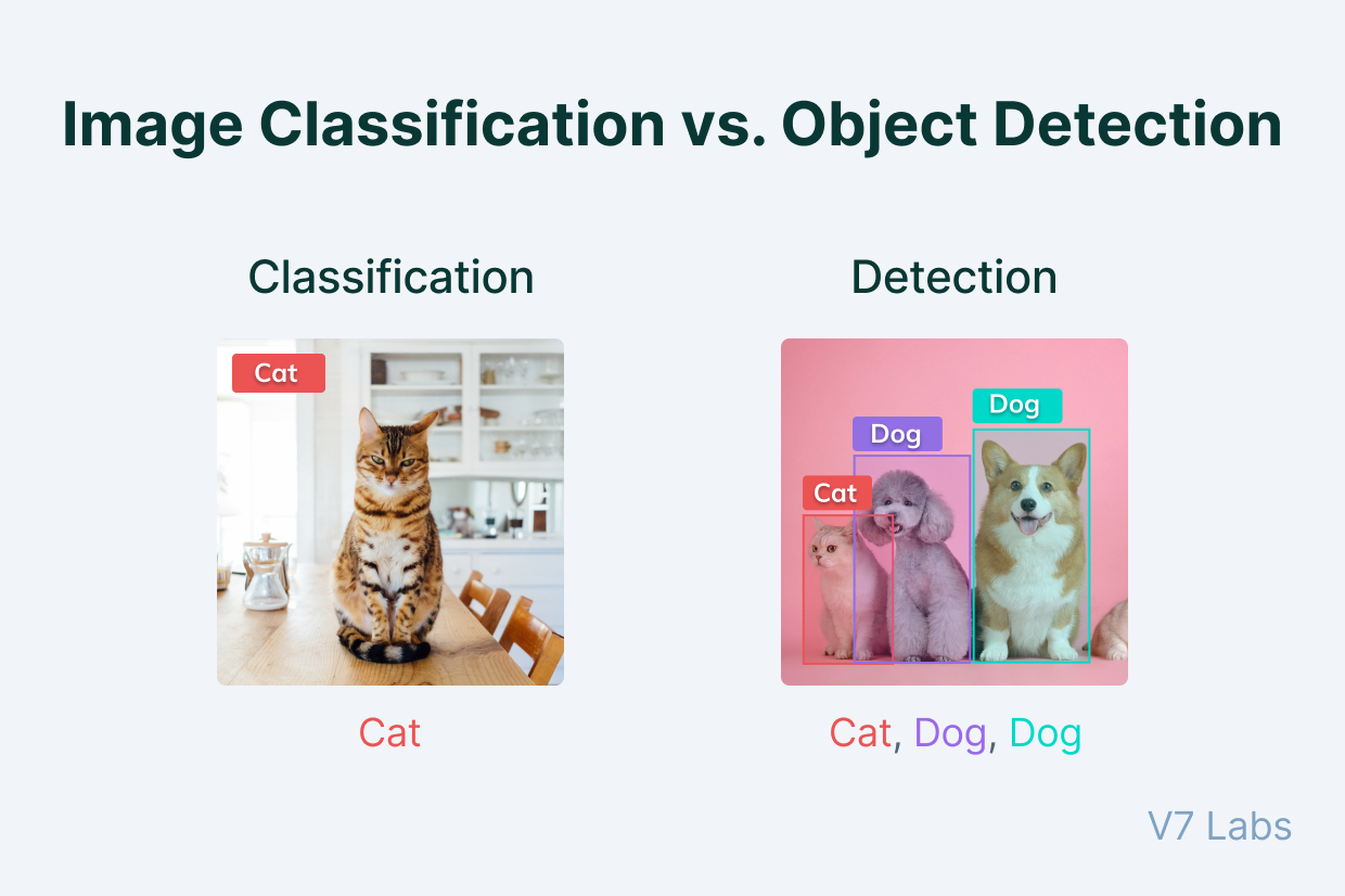
Object detection is an advanced task in the CV field that deals with the localization and classification of objects contained in an image or video. For easy understanding, let’s distinguish between image classification and object detection. Image classification sends a whole image through a classifier for it to spit out a tag. Classifiers take into consideration the whole image but don’t tell you where the tag appears in the image. Object detection is slightly more sophisticated, as it creates a bounding box around the classified object. Figure 1 illustrates this distinction.
From an ML perspective, object detection is a multi-task learning problem, the term that we discussed in a previous article. Specifically, the detectors are trained with a joined (simplified) objective function as below:
\[\mathcal{L}_{total} = \lambda_{loc}\mathcal{L}_{loc}(\widehat{b}, b) + \lambda_{cls}\mathcal{L}_{cls}(\widehat{y}, y)\]where $\widehat{b}$ and $b$ are predicted and ground truth bounding box coordinates, usually in the form of ($x_{min}$, $y_{min}$, $x_{max}$, $y_{max}$) or ($x_{center}$, $y_{center}$, $width$, $height$); $\widehat{y}$ and $y$ are the predicted probability and ground truth category of the object in that bounding box. \(\mathcal{L}_{loc}\) can be a simple IoU function, \(\mathcal{L}_{cls}\) can be a cross-entropy loss function; $\lambda_{loc}$ and $\lambda_{cls}$ are control hyper-parameters to balance these two loss terms.
Object detection models typically can be categorized into 2 groups:
- Two-stage (Proposal-based) detectors: The two stages of a two-stage detector can be divided by an RoI (Region of Interest) Pooling layer. One of the prominent two-stage object detectors is Faster R-CNN. It has the first stage called RPN, a Region Proposal Network to predict candidate bounding boxes. In the second stage, features are by RoI pooling operation from each candidate box for the following classification and bounding box regression tasks.
- One-stage (Proposal-free) detectors: In contrast, a one-stage detector predicts bounding boxes in a single step without using region proposals. It leverages the help of a grid box and anchors to localize the region of detection in the image and constraint the shape of the object. In this tutorial, I will use a YOLOv3 model, a popular one-stage detector, with the API implemented in PyTorch for demonstration, other architecture will be developed in the future.
2. Building an Object Detection Pipeline
In this section, we will walk through an end-to-end object detection pipeline, which is built in a similar way to any PyTorch classification pipeline.
VOC2007 Dataset
The VOC2007 dataset will be used, which contains 5011 images and 4952 images in the training set and test set, respectively. You can download the dataset from here. After downloading, you should organize the dataset as the below structure and then convert the provided labels to YOLO format.
│
├───datasets
│   └───VOC2007
│       ├───train
│       │   ├───images
│       │   │       2007_000005.jpg
│       │   │       ...
│       │   └───labels
│       │           2007_000005.xml
│       │           ...
│       └───val
│           ├───images
│           │       2007_000001.jpg
│           │       ...
│           └───labels
│                   2007_000001.xml
|                   ...
├───source
│   └───*.py
After organizing the dataset, as any PyTorch classification pipeline, we need to write a Dataset class with a __getitem__ function to return a pair of an image and its label (bounding boxes and classes). Snippet 1 illustrates the implementation.
"""
Snippet 1: Dataset class.
"""
from libs import *

class DetImageDataset(torch.utils.data.Dataset):
    def __init__(self,
        images_path, labels_path
        , image_size = 416
        , augment = False
        , multiscale = False
    ):
        self.image_files, self.label_files = sorted(glob.glob(images_path + "/*")), sorted(glob.glob(labels_path + "/*"))
        self.image_size = image_size
        self.augment = augment
        self.transforms = A.Compose(
            [
                A.HorizontalFlip(
                    p = 0.5,
                ),
                A.BBoxSafeRandomCrop(
                    erosion_rate = 0.2,
                    p = 0.5,
                ),
                A.RandomBrightnessContrast(
                    brightness_limit = 0.2, contrast_limit = 0.2,
                    p = 0.3,
                ),
                A.RGBShift(
                    r_shift_limit = 30, g_shift_limit = 30, b_shift_limit = 30,
                    p = 0.3,
                ),
            ],
            A.BboxParams("yolo", ["classes"])
        )
        self.multiscale = multiscale
        self.image_sizes = [self.image_size + 32*scale for scale in range(-1, 2)]

    def __len__(self,
    ):
        return len(self.image_files)

    def square_pad(self,
        image,
    ):
        _, h, w = image.shape
        gap_pad = np.abs(h - w)
        if h - w < 0:
            pad = (0, 0, gap_pad // 2, gap_pad - gap_pad // 2)
        else:
            pad = (gap_pad // 2, gap_pad - gap_pad // 2, 0, 0)

        image = F.pad(
            image,
            pad = pad, value = 0.0,
        )
        return image, [0] + list(pad)

    def __getitem__(self,
        index,
    ):
        image_file, label_file = self.image_files[index], self.label_files[index]
        image = cv2.imread(image_file)
        image = cv2.cvtColor(
            image,
            code = cv2.COLOR_BGR2RGB,
        )
        bboxes = np.loadtxt(label_file)
        bboxes = bboxes.reshape(-1, 5)
        if self.augment:
            Transformed = self.transforms(
                image = image,
                classes = bboxes[:, 0], bboxes = bboxes[:, 1:]
            )
            image = Transformed["image"]
            bboxes[:, 1:] = np.array(Transformed["bboxes"])

        image = torch.tensor(image)
        image = image.permute(2, 0, 1)
        _, h, w = image.shape
        image, pad = self.square_pad(image); _, padded_h, padded_w = image.shape
        c1, c2, c3, c4,  = w*(bboxes[:, 1] - bboxes[:, 3]/2) + pad[1], w*(bboxes[:, 1] + bboxes[:, 3]/2) + pad[2], h*(bboxes[:, 2] - bboxes[:, 4]/2) + pad[3], h*(bboxes[:, 2] + bboxes[:, 4]/2) + pad[4],
        bboxes[:, 1], bboxes[:, 2], bboxes[:, 3], bboxes[:, 4],  = ((c1 + c2)/2)/padded_w, ((c3 + c4)/2)/padded_h, bboxes[:, 3]*(w/padded_w), bboxes[:, 4]*(h/padded_h),
        return image.float(), F.pad(
            torch.tensor(bboxes),
            pad = (1, 0, 0, 0), value = 0.0,
        )

    def collate_fn(self,
        batch,
    ):
        images, labels = list(zip(*batch))
        if self.multiscale and np.random.random() <= 0.1:
            self.image_size = np.random.choice(self.image_sizes)
        images = torch.stack([
            F.interpolate(
                image.unsqueeze(0),
                self.image_size, mode = "nearest",
            ).squeeze(0) for image in images
        ])
        images = images/255

        labels = [bboxes for bboxes in labels if bboxes is not None]
        for index, bboxes in enumerate(labels):
            bboxes[:, 0] = index
        if len(labels) != 0:labels = torch.cat(labels)
        return images, labels
The component that I want you to notice in the above implementation is self.transforms, which is used for performing data augmentation. Here, I use the Albumentations library, you can modify the self.transforms attribute to use the data augmentation strategy that you want depending on your problem. You can also change the image size or multi-scale training strategy easily.
Config the model
The next step is to config the YOLO model and set the training hyper-parameters. This is an easy step. Based on the provided yolov3.cfg, we just need to change some hyper-parameters we will use. For example, I changed the number of epochs, learning rate, and weight decay as below:
num_epochs=250

lr=0.0001
weight_decay=0.0005
A Training Function
Next, in any PyTorch classification pipeline, we need a training function. The implementation of this function in Snippet 2 added a feature that returns loss and mAP from training and evaluation at each epoch. This feature is usually ignored in many open-source repositories.
"""
Snippet 2: Training function.
"""
from libs import *

def train_fn(
    train_loaders,
    model,
    num_epochs,
    optimizer,
    lr_scheduler,
    save_ckp_dir = "./",
    training_verbose = True,
):
    print("\nStart Training ...\n" + " = "*16)
    model = model.cuda()

    best_map = 0
    for epoch in tqdm.tqdm(range(1, num_epochs + 1), disable = training_verbose):
        if training_verbose:
            print("epoch {:2}/{:2}".format(epoch, num_epochs) + "\n" + " - "*16)
        if epoch <= int(0.08*num_epochs):
            for param_group in optimizer.param_groups:
                param_group["lr"] = model.hyperparams["lr"]*epoch/(int(0.08*num_epochs))
        else:
            lr_scheduler.step()
        wandb.log(
            {"lr":optimizer.param_groups[0]["lr"]},
            step = epoch,
        )
        model.train()
        running_loss = 0.0
        for images, labels in tqdm.tqdm(train_loaders["train"], disable = not training_verbose):
            images, labels = images.cuda(), labels.cuda()

            logits = model(images)
            loss = compute_loss(
                logits, labels,
                model,
            )[0]

            loss.backward()
            optimizer.step(), optimizer.zero_grad()

            running_loss = running_loss + loss.item()*images.size(0)
        train_loss = running_loss/len(train_loaders["train"].dataset)
        wandb.log(
            {"train_loss":train_loss},
            step = epoch,
        )
        if training_verbose:
            print("train - loss:{:.4f}".format(train_loss))

        with torch.no_grad():
            model.eval()
            running_classes, running_statistics = [], []
            for images, labels in tqdm.tqdm(train_loaders["val"], disable = not training_verbose):
                images, labels = images.cuda(), labels.cuda()
                labels[:, 2:] = xywh2xyxy(labels[:, 2:])
                labels[:, 2:] = labels[:, 2:]*int(train_loaders["val"].dataset.image_size)

                logits = model(images)
                logits = non_max_suppression(
                    logits,
                    conf_thres = 0.1, iou_thres = 0.5,
                )

                running_classes, running_statistics = running_classes + labels[:, 1].tolist(), running_statistics + get_batch_statistics(
                    [logit.cpu() for logit in logits], labels.cpu(),
                    0.5,
                )
        val_map = ap_per_class(
            *[np.concatenate(stats, 0) for stats in list(zip(*running_statistics))],
            running_classes,
        )[2].mean()
        wandb.log(
            {"val_map":val_map},
            step = epoch,
        )
        if training_verbose:
            print("val - map:{:.4f}".format(val_map))
        if best_map < val_map:
            best_map = val_map; torch.save(model, "{}/yolov3.ptl".format(save_ckp_dir))
Let’s notice at arguments that the above function receives, optimizer and lr_scheduler in particular. You can create any optimizer such as SGD or Adam, any lr_scheduler such as StepLR or CosineAnnealingLR, and pass them into the function, then the function will do all the rest.
Start training
Now, we are ready to train our YOLO model. Firstly, let’s initialize PyTorch data loaders:
"""
Snippet 3: Data Loaders.
"""
datasets = {
    "train":DetImageDataset(
        images_path = "../datasets/{}/train/images".format(args.dataset), labels_path = "../datasets/{}/train/labels".format(args.dataset)
        , image_size = 416
        , augment = True
        , multiscale = True
    ),
    "val":DetImageDataset(
        images_path = "../datasets/{}/val/images".format(args.dataset), labels_path = "../datasets/{}/val/labels".format(args.dataset)
        , image_size = 416
        , augment = False
        , multiscale = False
    ),
}
train_loaders = {
    "train":torch.utils.data.DataLoader(
        datasets["train"], collate_fn = datasets["train"].collate_fn,
        num_workers = 8, batch_size = 32,
        shuffle = True,
    ),
    "val":torch.utils.data.DataLoader(
        datasets["val"], collate_fn = datasets["val"].collate_fn,
        num_workers = 8, batch_size = 32,
        shuffle = False,
    ),
}
Next, we will initialize a YOLO model, load pre-trained backbone weighs, and create an optimizer and a lr_scheduler:
"""
Snippet 4: Model Initialization.
"""
model = Darknet("pytorchyolo/configs/yolov3.cfg")
model.load_darknet_weights("../ckps/darknet53.conv.74")
optimizer = optim.Adam(
    model.parameters(),
    lr = model.hyperparams["lr"], weight_decay = model.hyperparams["weight_decay"],
)
lr_scheduler = optim.lr_scheduler.CosineAnnealingLR(
    optimizer,
    eta_min = 0.01*model.hyperparams["lr"], T_max = int(0.92*int(model.hyperparams["num_epochs"])),
)
Finally, start training. Don’t forget to use wandb to log the results:
"""
Snippet 5: Training.
"""
wandb.login()
wandb.init(
    project = "ezdet", name = args.dataset,
)
save_ckp_dir = "../ckps/{}".format(args.dataset)
if not os.path.exists(save_ckp_dir):
    os.makedirs(save_ckp_dir)
train_fn(
    train_loaders,
    model,
    num_epochs = int(model.hyperparams["num_epochs"]),
    optimizer = optimizer,
    lr_scheduler = lr_scheduler,
    save_ckp_dir = save_ckp_dir,
)
wandb.finish()
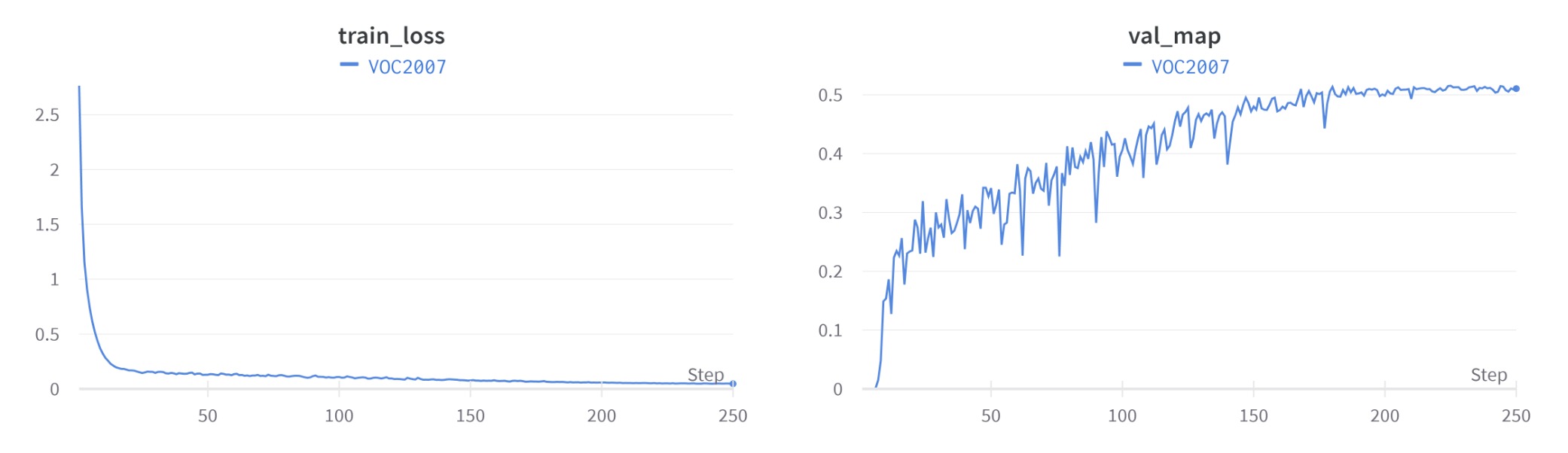
3. Results
If you carefully follow this tutorial, the results will be like this:
4. Integrating ezdet into other ML projects
As mentioned above, the ezdet repository can be easily integrated into other ML projects. To demonstrate that, I have used ezdet and Flower to train YOLOv3 models in a Federated Learning setting. Let’s check the full implementation here.
Stay tuned for more content …
References
[1] The Ultimate Guide to Object Detection
[2] Bibliometric Analysis of One-stage and Two-stage Object Detection
Comments